I wish to reproduce a very informative plot in google
Given a group of samples and a list of genes for which we have data how each genes has mutated and whether the alleles are homozygous of heterozygous. These are expressed as boolean values
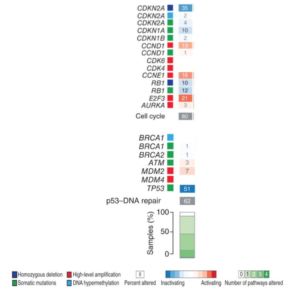
Genes enriched in 2 pathways like cell cycle and p53 as shown in this figure
Map of functional alterations for a group of patients. Genes (rows) encoding components p53–DNA repair pathway; are affected by selected functional events (percent of samples altered and types of alteration are represented by colored squares) across group of samples in column. Alterations of the pathway are observed stacked green bar plots at bottom
I have the boolean matrix of mutated genes per sample would be grateful for assistence.
An example of my copy number data
> dataset_gistic$annotations
     type                event
G2   "Homozygous Deletion"   "ACVR2A"
G13  "Homozygous Deletion"   "HIST1H3B"
G73  "Heterozygous Deletion" "CCNE1"
G74  "Heterozygous Deletion" "TSHZ3"
G78  "Low-level Amplification"    "CTNNB1"
G110 "Low-level Amplification"    "CCNE1"
G111 "Low-level Amplification"    "TSHZ3"
G119 "High-level Amplification"   "PIK3CA"
G121 "High-level Amplification"   "NIPBL"
G147 "High-level Amplification"   "CCNE1"
G148 "High-level Amplification"   "TSHZ3"
>

> dput(dataset_gistic$annotations)
structure(c("Homozygous Loss", "Homozygous Loss", "Homozygous Loss",
"Homozygous Loss", "Homozygous Loss", "Homozygous Loss", "Heterozygous Loss",
"Heterozygous Loss", "Heterozygous Loss", "Heterozygous Loss",
"Heterozygous Loss", "Heterozygous Loss", "Heterozygous Loss",
"Heterozygous Loss", "Heterozygous Loss", "Heterozygous Loss",
"Heterozygous Loss", "Heterozygous Loss", "Heterozygous Loss",
"Heterozygous Loss", "Heterozygous Loss", "Heterozygous Loss",
"Heterozygous Loss", "Heterozygous Loss", "Heterozygous Loss",
"Heterozygous Loss", "Heterozygous Loss", "Heterozygous Loss",
"Heterozygous Loss", "Heterozygous Loss", "Heterozygous Loss",
"Heterozygous Loss", "Heterozygous Loss", "Heterozygous Loss",
"Heterozygous Loss", "Heterozygous Loss", "Heterozygous Loss",
"Heterozygous Loss", "Heterozygous Loss", "Heterozygous Loss",
"Heterozygous Loss", "Low-level Gain", "Low-level Gain", "Low-level Gain",
"Low-level Gain", "Low-level Gain", "Low-level Gain", "Low-level Gain",
"Low-level Gain", "Low-level Gain", "Low-level Gain", "Low-level Gain",
"Low-level Gain", "Low-level Gain", "Low-level Gain", "Low-level Gain",
"Low-level Gain", "Low-level Gain", "Low-level Gain", "Low-level Gain",
"Low-level Gain", "Low-level Gain", "Low-level Gain", "Low-level Gain",
"Low-level Gain", "High-level Gain", "High-level Gain", "High-level Gain",
"High-level Gain", "High-level Gain", "High-level Gain", "High-level Gain",
"High-level Gain", "High-level Gain", "High-level Gain", "High-level Gain",
"High-level Gain", "ACVR2A", "HIST1H3B", "CDKN2A", "PTEN", "NAV3",
"LIN7A", "ARID1A", "ACVR2A", "SCN3A", "CTNNB1", "PBRM1", "EPHA3",
"POLQ", "PIK3CA", "SLIT2", "NIPBL", "MSH3", "APC", "HIST1H3B",
"ARID1B", "CDKN2A", "NOTCH1", "PTEN", "CCND1", "KRAS", "LRRK2",
"ARID2", "NAV3", "LIN7A", "SIN3A", "TP53", "ERBB2", "GPATCH8",
"RNF43", "GATA6", "SMAD4", "CCDC102B", "STK11", "SMARCA4", "CCNE1",
"TSHZ3", "CTNNB1", "PIK3CA", "SLIT2", "NIPBL", "HIST1H3B", "ARID1B",
"EGFR", "KCNQ3", "NOTCH1", "PTEN", "CCND1", "KRAS", "LRRK2",
"ARID2", "SIN3A", "ERBB2", "GPATCH8", "RNF43", "GATA6", "CCDC102B",
"STK11", "SMARCA4", "CCNE1", "TSHZ3", "PIK3CA", "NIPBL", "EGFR",
"KCNQ3", "CCND1", "KRAS", "ERBB2", "GPATCH8", "RNF43", "GATA6",
"CCNE1", "TSHZ3"), .Dim = c(77L, 2L), .Dimnames = list(c("G2",
"G13", "G17", "G19", "G24", "G25", "G38", "G39", "G40", "G41",
"G42", "G43", "G44", "G45", "G46", "G47", "G48", "G49", "G50",
"G51", "G54", "G55", "G56", "G57", "G58", "G59", "G60", "G61",
"G62", "G63", "G64", "G65", "G66", "G67", "G68", "G69", "G70",
"G71", "G72", "G73", "G74", "G78", "G82", "G83", "G84", "G87",
"G88", "G89", "G90", "G92", "G93", "G94", "G95", "G96", "G97",
"G100", "G102", "G103", "G104", "G105", "G107", "G108", "G109",
"G110", "G111", "G119", "G121", "G126", "G127", "G131", "G132",
"G139", "G140", "G141", "G142", "G147", "G148"), c("type", "event"
)))
>
And this is sample of my mutational data the number of mutations for each gene in each sample
    om$numericMatrix
       LP6005500-DNA_D03 LP6008336-DNA_G01 LP6008460-DNA_D01 LP6005334-DNA_H01
TP53                   2                 2                 2                 2
CDKN2A                 3                 1                 2                 0
       LP6007600 LP6008334-DNA_A03 LP6008334-DNA_A04 LP6008334-DNA_B02
TP53           2                 2                 2                 2
CDKN2A         0                 0                 0                 0
       LP6008334-DNA_C02 LP6008334-DNA_D02 LP6008336-DNA_H01 LP6008337-DNA_A07
TP53                   2                 1                 2                 2
CDKN2A                 0                 0                 0                 0
       LP6008337-DNA_H06 LP6008460-DNA_A04
TP53                   2                 2
CDKN2A                 0                 0
>

> dput(om$numericMatrix)
structure(c(2, 3, 2, 1, 2, 2, 2, 0, 2, 0, 2, 0, 2, 0, 2, 0, 2,
0, 1, 0, 2, 0, 2, 0, 2, 0, 2, 0), .Dim = c(2L, 14L), .Dimnames = list(
    c("TP53", "CDKN2A"), c("LP6005500-DNA_D03", "LP6008336-DNA_G01",
    "LP6008460-DNA_D01", "LP6005334-DNA_H01", "LP6007600", "LP6008334-DNA_A03",
    "LP6008334-DNA_A04", "LP6008334-DNA_B02", "LP6008334-DNA_C02",
    "LP6008334-DNA_D02", "LP6008336-DNA_H01", "LP6008337-DNA_A07",
    "LP6008337-DNA_H06", "LP6008460-DNA_A04")))
>


dput()will help us "reproduce" your input data. If you invest a couple of minutes going through the link and subsequently increase the "quality" and "completeness" of your questions, you will get answers much faster you do now. $\endgroup$